Mastering Excel means mastering excel formulas. These 100 formulas are essential for data analysis, finance, planning, reporting, dashboards, business management, HR, accounting, and everyday office use. Each formula below includes its purpose, syntax, and an example you can copy into Excel.
1. SUM
Purpose: Adds numbers in a range.
Structure: =SUM(number1, number2, ...)
Example: = SUM(B2:B4)
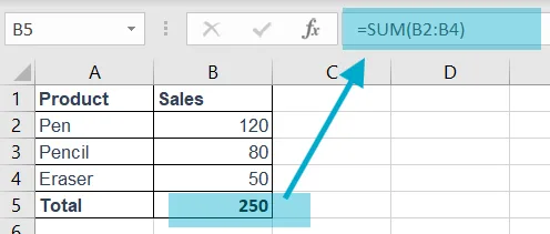
Explanation: Adds 120+80+50 = 250.
The SUM function is also easy to pick from Excel built-in function quickly. See below image shown how to pick the Sum() function from Home ribbon > AutoSum. It also can be inserted by pressing Alt+= on keyboard.

2. AVERAGE
Purpose: Returns the average value of numbers.
Structure: =AVERAGE(range)
Example: =AVERAGE(B1:B3)
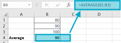
Explanation: (80+90+100)/3 = 90.
The AVERAGE function is also easy to pick from Excel built-in function quickly. It can be found below of the Sum() function at Home ribbon > AutoSum.
3. COUNT
Purpose: Counts numeric cells.
Structure: =COUNT(range)
Example: =COUNT(C2:C8)
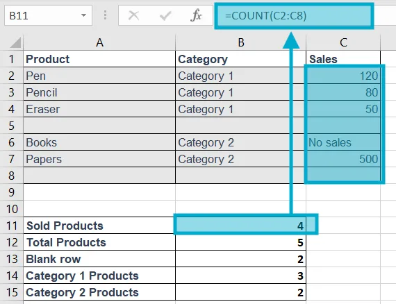
Explanation: Counts only numbers.
The COUNT function is also easy to pick from Excel built-in function quickly. It can be found below of the Sum() function at Home ribbon > AutoSum.
4. COUNTA
Purpose: Counts non-empty cells.
Structure: =COUNTA(range)
Example: =COUNTA(C2:C8)
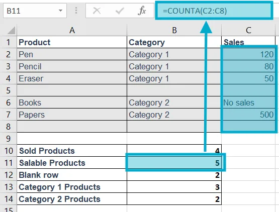
Explanation: Text and numbers both counted.
5. COUNTBLANK
Purpose of this Excel formula: Counts blank cells.
Structure: =COUNTBLANK(range)
Example: =COUNTBLANK(C2:C8)
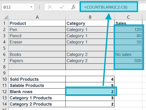
Explanation: Shows how many cells are empty.
6. COUNTIF
Purpose of this Excel formula: Counts cells matching one condition.
Structure: =COUNTIF(range, criteria)
Example: =COUNTIF(B1:B8, "Category 1")
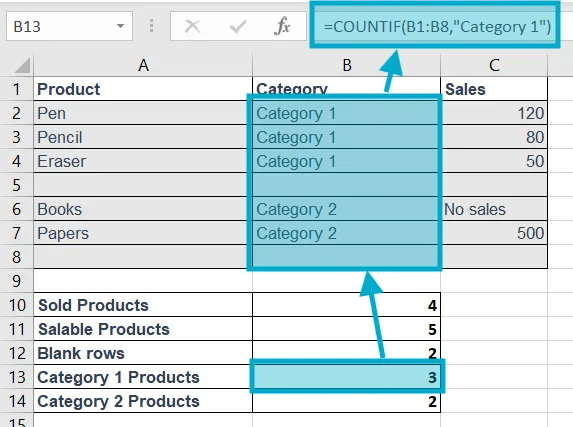
Explanation: to count how many products that have in Category 1, we used this formula =COUNTIF(B1:B8,"Category 1")
7. COUNTIFS
Purpose of this Excel formula: Counts cells meeting multiple conditions.
Structure: =COUNTIFS(range1,criteria1,range2,criteria2,...)
Example: =COUNTIFS(B1:B8,"Category 1",C1:C8,">100")
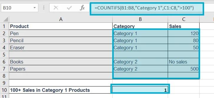
Explanation: to count how many products that have 100+ sales records in Category 1, we used this formula =COUNTIFS(B1:B8,"Category 1",C1:C8,">100")
8. SUMIF
Purpose of this Excel formula: Adds numbers based on one condition.
Structure: =SUMIF(range, criteria, sum_range)
Example: =SUMIF(B2:B14,F2,D2:D14)

Explanation: on cell G2, we wanted to get total sales of product “Pen”. So we use the formula =SUMIF(B2:B14,F2,D2:D14).
Here, range B2:B14 contain Product names, criteria is Pen (cell F2) which will be searched in range B2:B14. We may write “Pen” instead of using cell F2 in the the formula. Then the sum_range D2:D14 contain Sales records from there we got conditional SUM result 360 of Total Sales of Pen.
9. SUMIFS
Purpose of this Excel formula: Adds numbers based on multiple conditions.
Structure: =SUMIFS(sum_range, range1,criteria1,...)
Example: =SUMIFS(D2:D14,C2:C14,F2,A2:A14,G2)
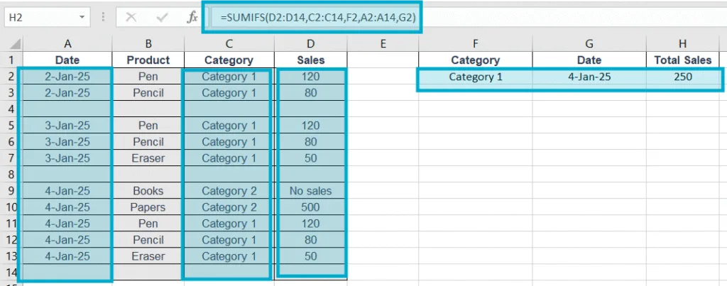
Explanation: on cell H2, we wanted to get total sales based on Category and Date as mentioned. so we use the formula =SUMIFS(D2:D14,C2:C14,F2,A2:A14,G2)
Here, sum_range D2:D14 contain Sales records, F2 is criteria1 which will be searched in range1 C2:C14. We may write “Category 1” instead of using cell F2 in the the formula’s criteria1. G2 is criteria2 which will be searched in range2 A2:A14. We may write a specific date “4-Jan-25” instead of using cell D2 in the the formula’s criteria2.
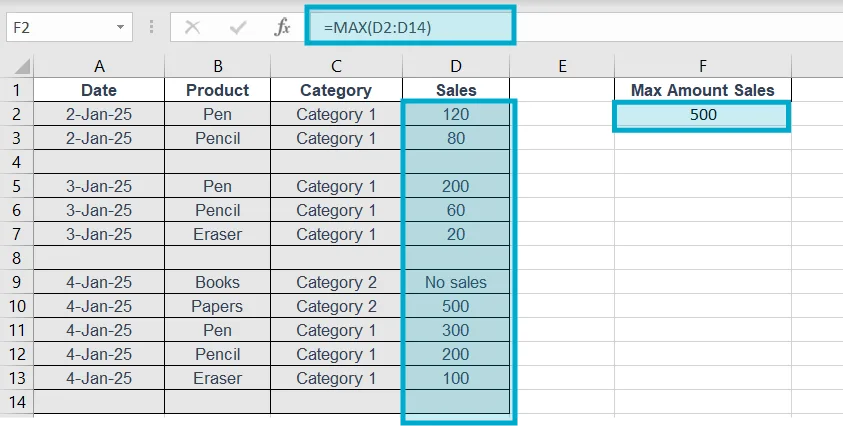
11. MAX
Purpose of this Excel formula: Shows largest value.
Structure: =MAX(range)
Example: =MAX(D2:D14)
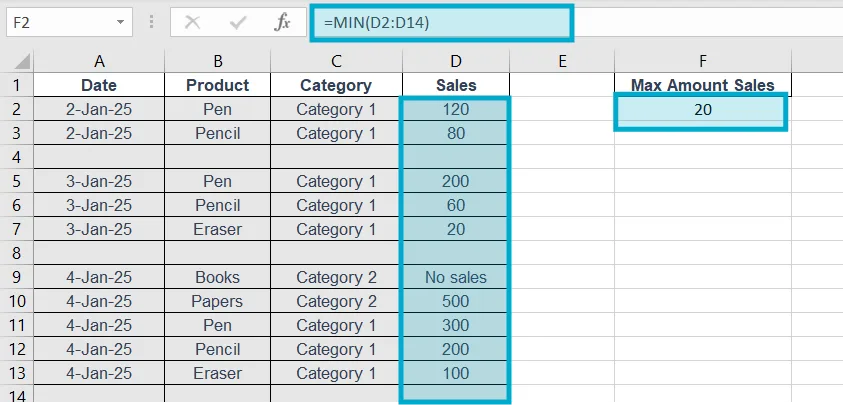
11. MIN
Purpose of this Excel formula: Shows smallest value.
Structure: =MIN(range)
Example: =MIN(D2:D14)
12. LARGE
Purpose of this Excel formula: Returns nth largest number.
Structure: =LARGE(range,n)
Example: =LARGE(D2:D14,2)
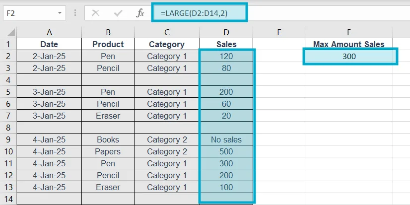
Explanation: If we wanted to get a specific (nth) LARGE number, then we can use this formula. Here, we wanted to see 2nd large number on the Sales (D) columns.
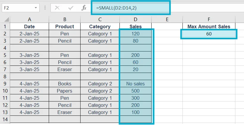
13. SMALL
Purpose of this Excel formula: Returns nth smallest number.
Structure: =SMALL(range,n)
Example: =SMALL(D2:D14,2)
14. PRODUCT
Purpose of this Excel formula: Multiplies all numbers.
Structure: =PRODUCT(range)
15. SQRT
Purpose of this Excel formula: Square root.
Structure: =SQRT(number)
16. POWER
Purpose of this Excel formula: Exponent calculation.
Structure: =POWER(number,power)
17. ABS
Purpose of this Excel formula: Absolute value (removes negative sign).
Structure: =ABS(number)
18. RAND
Purpose: Random decimal between 0–1.
Structure: =RAND()
19. RANDBETWEEN
Purpose: Random integer in range.
Structure: =RANDBETWEEN(bottom, top)
20. MOD
Purpose: Remainder after division.
Structure: =MOD(number, divisor)
Example: =MOD(7,2) → 1.
21. IF
Purpose: Returns different results based on condition.
Structure: =IF(logical_test,true_result,false_result)
Example: =IF(A1>=50,"Pass","Fail")
22. IFERROR
Purpose: Replace errors with a message.
Structure: =IFERROR(value, value_if_error)
Example: =IFERROR(A1/B1,"Invalid")
23. AND
Purpose: Result is TRUE when all conditions are true.
Structure: =AND(condition1,condition2)
24. OR
Purpose: TRUE if any condition is TRUE.
Structure: =OR(condition1,condition2)
25. NOT
Purpose: Reverses TRUE/FALSE.
Structure: =NOT(condition)
26. XOR
Purpose: TRUE if only one condition is true.
Structure: =XOR(condition1,condition2)
27. CONCAT
Purpose: Joins text.
Structure: =CONCAT(text1,text2,...)
28. TEXTJOIN
Purpose: Joins text with delimiter.
Structure: =TEXTJOIN(delimiter,ignore_empty,range)
29. LEFT
Purpose: Extracts text from the left.
Structure: =LEFT(text,num_chars)
30. RIGHT
Purpose: Extracts from right.
Structure: =RIGHT(text,num_chars)
31. MID
Purpose: Extracts text from the middle.
Structure: =MID(text,start_num,num_chars)
32. LEN
Purpose: Counts characters.
Structure: =LEN(text)
33. TRIM
Purpose: Removes extra spaces.
Structure: =TRIM(text)
34. LOWER
Purpose: Converts to lowercase.
Structure: =LOWER(text)
35. UPPER
Purpose: Converts to uppercase.
Structure: =UPPER(text)
36. PROPER
Purpose: Capitalizes each word.
Structure: =PROPER(text)
37. REPLACE
Purpose: Replace characters by position.
Structure: =REPLACE(old,start,num,new)
38. SUBSTITUTE
Purpose: Replace specific text.
Structure: =SUBSTITUTE(text,old,new)
39. FIND
Purpose: Find position (case-sensitive).
Structure: =FIND(find_text,within_text)
40. SEARCH
Purpose: Find position (not case-sensitive).
Structure: =SEARCH(find_text,within_text)
41. TEXT
Purpose: Format numbers as text.
Structure: =TEXT(value,format_text)
42. VLOOKUP
Purpose: Lookup a value vertically.
Structure: =VLOOKUP(lookup_value,table,col,range_lookup)
Example grid:
| A | B |
|---|---|
| Pen | 120 |
| Pencil | 80 |
| Eraser | 50 |
=VLOOKUP("Pen",A1:B4,2,FALSE) → 120.
43. HLOOKUP
Purpose: Horizontal lookup.
Structure: =HLOOKUP(value,table,row_index,range_lookup)
44. XLOOKUP
Purpose: Modern replacement for VLOOKUP.
Structure:=XLOOKUP(lookup_value,lookup_array,return_array,not_found)
45. INDEX
Purpose: Return value from row/column.
Structure: =INDEX(array,row_num,column_num)
46. MATCH
Purpose: Position of value.
Structure: =MATCH(lookup_value,lookup_array,match_type)
47. INDEX + MATCH
Purpose: More flexible lookup.
Example: =INDEX(B2:B5,MATCH("Pen",A2:A5,0))
48. CHOOSE
Purpose: Select value by index.
Structure: =CHOOSE(index,value1,value2,...)
49. OFFSET
Purpose: Reference cell shifted from starting cell.
Structure: =OFFSET(reference,rows,cols)
50. INDIRECT
Purpose: Convert text to cell reference.
Structure: =INDIRECT(text_reference)
51. ADDRESS
Purpose: Returns cell address.
Structure: =ADDRESS(row,col)
52. ROW
Purpose: Return row number.
Structure: =ROW(reference)
53. COLUMN
Purpose: Return column number.
Structure: =COLUMN(reference)
54. TRANSPOSE
Purpose: Convert rows to columns and vice versa.
Structure: =TRANSPOSE(array)
55. TODAY
Purpose: Returns today’s date.
Structure: =TODAY()
56. NOW
Purpose: Returns date and time.
Structure: =NOW()
57. DAY
Purpose: Extract day number.
Structure: =DAY(date)
58. MONTH
Purpose: Extract month.
Structure: =MONTH(date)
59. YEAR
Purpose: Extract year.
Structure: =YEAR(date)
60. DATE
Purpose: Create a date.
Structure: =DATE(year,month,day)
61. DATEDIF
Purpose: Days/months/years between dates.
Structure: =DATEDIF(start,end,unit)
62. WEEKDAY
Purpose: Returns day of week.
Structure: =WEEKDAY(date)
63. EOMONTH
Purpose: End of month date.
Structure: =EOMONTH(start_date,months)
64. NETWORKDAYS
Purpose: Working days between dates.
Structure: =NETWORKDAYS(start,end)
65. WORKDAY
Purpose: Returns future working date.
Structure: =WORKDAY(start,days)
66. TIME
Purpose: Construct time.
Structure: =TIME(hour,minute,second)
67. HOUR
Purpose: Extract hour.
Structure: =HOUR(time)
68. MINUTE
Purpose: Extract minute.
Structure: =MINUTE(time)
69. SECOND
Purpose: Extract second.
Structure: =SECOND(time)
70. ROUND
Purpose: Round to decimals.
Structure: =ROUND(number,decimals)
71. ROUNDUP
Purpose: Round upward.
Structure: =ROUNDUP(number,decimals)
72. ROUNDDOWN
Purpose: Round downward.
Structure: =ROUNDDOWN(number,decimals)
73. INT
Purpose: Remove decimal.
Structure: =INT(number)
74. CEILING
Purpose: Round up to nearest multiple.
Structure: =CEILING(number,multiple)
75. FLOOR
Purpose: Round down to nearest multiple.
Structure: =FLOOR(number,multiple)
76. EVEN
Purpose: Round up to nearest even number.
Structure: =EVEN(number)
77. ODD
Purpose: Round up to nearest odd number.
Structure: =ODD(number)
78. AVERAGEIF
Purpose: Average by one condition.
Structure: =AVERAGEIF(range,criteria,average_range)
79. AVERAGEIFS
Purpose: Average by multiple conditions.
Structure: =AVERAGEIFS(average_range,range1,criteria1,...)
80. MEDIAN
Purpose: Middle value.
Structure: =MEDIAN(range)
81. MODE
Purpose: Most frequent value.
Structure: =MODE(range)
82. STDEV
Purpose: Standard deviation.
Structure: =STDEV(range)
83. VAR
Purpose: Variance.
Structure: =VAR(range)
84. CORREL
Purpose: Correlation between datasets.
Structure: =CORREL(array1,array2)
85. PMT
Purpose: Loan monthly payment.
Structure: =PMT(rate,nper,pv)
86. FV
Purpose: Future value.
Structure: =FV(rate,nper,pmt,pv)
87. PV
Purpose: Present value.
Structure: =PV(rate,nper,pmt,fv)
88. NPV
Purpose: Net present value.
Structure: =NPV(rate,values)
89. IRR
Purpose: Internal rate of return.
Structure: =IRR(values)
90. RATE
Purpose: Interest rate.
Structure: =RATE(nper,pmt,pv,fv)
91. UNIQUE
Purpose: Returns unique items.
Structure: =UNIQUE(range)
92. FILTER
Purpose: Filter rows by condition.
Structure: =FILTER(range,include)
93. SORT
Purpose: Sort range.
Structure: =SORT(range,sort_index,order)
94. SORTBY
Purpose: Sort based on another column.
Structure: =SORTBY(range,by_array,order)
95. SEQUENCE
Purpose: Generate sequence numbers.
Structure: =SEQUENCE(rows,cols,start,step)
96. RANDARRAY
Purpose: Random array.
Structure: =RANDARRAY(rows,cols,min,max,integer)
97. XMATCH
Purpose: Advanced MATCH.
Structure: =XMATCH(lookup_value,lookup_array,match_mode)
98. LET
Purpose: Assign variables inside formula.
Structure: =LET(name,value,calculation)
99. LAMBDA
Purpose: Create custom functions.
Structure: =LAMBDA(parameters,formula)(arguments)
100. HYPERLINK
Purpose: Create clickable link.
Structure: =HYPERLINK(link,text)
Conclusion
These 100 Excel formulas cover everything from basic math to advanced analytics, dashboards, finance, HR, and data automation. Mastering these will make you a true Excel expert capable of handling any business or data problem.
If you want training, dashboards, templates, automated spreadsheets, or consultation, visit SoluExcel.com where complex data becomes clear and manageable.
To get Microsoft Excel, visit https://www.microsoft.com/en-us/microsoft-365/excel